===================================================================
Note: The following is an edited version of my original post. Thanks to Nick Edmonds for pointing out an inconsistency in my earlier analysis. Nick's comment forced me to think through the properties of my model more carefully. In light of his observation, I have modified the original model to include capital investment. My earlier conclusions remain unchanged.
===================================================================
I should have known better than to reason from accounting identities. But that's basically what I did in my last post and Nick Rowe called me out on it here. So I decided to go back and think through the exercise I had in mind using a simple model economy.
Consider a simple OLG model, with 2-period-lived agents. The young are endowed with output, y. Let N denote the number of young agents (normalize N=1). The young care only about consumption when they are old (hence, they save all their income y when young). Agents are risk-averse, with expected utility function E[u(c)]. There is a storage technology. If a young agent saves k units of output when young, he gets x*f(k) units of output in the next period, where x is a productivity parameter and f(.) is an increasing and strictly concave function (there are diminishing returns to capital accumulation). Assume that capital depreciates fully after it is used in production.
If x*f'(y) > 1, the economy is dynamically efficient. If x*f'(y) < 1, the economy is dynamically inefficient (and there is a welfare-enhancing role for government debt).
Now, imagine that there are two such economies, each in a separate location. Moreover, suppose that a known fraction 0 < s < 1 of young agents from each location migrate to the "foreign" location. The identity of who migrates is not known beforehand, so there is idiosyncratic risk, but no aggregate risk.
Next, assume that there are two other assets, money and bonds, both issued by the government supply (and endowed to the initial old). Let M be the supply of money, and let B denote the supply of bonds. Let D denote the total supply of nominal government debt:
[1] D = M + B
Money is a perpetuity that pays zero nominal interest. Bonds are one-period risk-free claims to money. (Once the bonds pay off, the government just re-issues a new bond offering B to suck cash back out of the system.) Assume that the government keeps D constant maintains a fixed bond/money ratio z = B/M, so that [1] can be written as:
[2] D = (1+z)*M
In what follows, I will keep D constant throughout and consider the effect of changing z (once and for all). Note, I am comparing steady-states here. Also, since D and M remain constant over time, and since there is no real growth in this economy, I anticipate that the steady state inflation rate will be equal to zero.
Let R denote the gross nominal interest rate (also the real interest rate, since inflation is zero). Assume that the government finances the carrying cost of its interest-bearing debt with a lump-sum tax,
[3] T = (R-1)*B
The difference between money and bonds is that bonds (or intermediated claims to bonds) cannot be transported across locations. Only money is transportable. The effect of this assumption is to impose a cash-in-advance constraint (CIA) on the young agents who move across locations. (Hence, we can interpret the relocation shock as an idiosyncratic liquidity shock).
Young agents are confronted with a portfolio allocation problem. Let P denote the price level. Since the young do not consume, they save their entire nominal income, P*y. Savings can be allocated to money, bonds, or capital,
[4] P*y = M + B + P*k
There is a trade off here: money is more liquid, but bonds and capital (generally) pay a higher return. The portfolio choice must be made before the young realize their liquidity shock.
Because there is idiosyncratic liquidity risk, the young can be made better off by pooling arrangement that we can interpret as a bank. The bank issues interest-bearing liabilities, redeemable for cash on demand. It uses these liabilities to finance its assets, M+B+P*k. Interest is only paid on bank liabilities that are left to mature into the next period. (The demandable nature of the debt can be motivated by assuming that the idiosyncratic shock is private information. It is straightforward to show that truth-telling here in incentive-compatible.)
Let me describe how things work here. Consider one of the locations. It will consist of two types of old agents: domestics and foreigners. The old foreigners use cash to buy output from the domestic young agents. The old domestics use banknotes to purchase output from the young domestics (the portion of the banknotes that turn into cash as the bond matures). The remaining banknotes can be redeemed for a share of the output produced by the maturing capital project. The old domestic agents must also pay a lump-sum tax.
As for the young in a given location, they accumulate cash equal to the sales of output to the old. After paying their taxes, the old collectively have cash balances equal to D. The young deposit this cash in their bank. The bank holds some cash back as reserves M and uses the rest to purchase newly-issued bonds B. The bank also uses some of its banknotes to purchase output P*k from the young workers, which the bank invests. At the end of this operation, the bank has assets M+B+P*k and a corresponding set of (demandable) liabilities. The broad money supply in this model is equal to M1 = M+B+P*k. The nominal GDP is given by NGDP = P*y + P*x*f(k).
Formally, I model the bank as a coalition of young agents. The coalition maximizes the expected utility of a representative member: (1-s)*u(c1) + s*u(c2), where c1 is consumption in the domestic location and c2 is consumption in the foreign location. The maximization above is constrained by condition [4] which, expressed in real terms, can be stated as:
[5] y = m + b + k
where m = M/P and b = B/P (real money and bond holdings, respectively).
In addition, there is a budget constraint:
[6] (1-s)*c1 + s*c2 = x*f(k) + R*b + m - t
where t = T/P (see condition [3]).
Finally, there is the "cash-in-advance" (CIA) constraint:
[7] s*c2 <= m
Note: the CIA constraint represents the "cash reserves" the bank has to set aside to meet expected redemptions. Because there is no aggregate risk here, the aggregate withdrawal amount is perfectly forecastable. This constraint may or may not bind. It will bind if the nominal interest rate is positive (i.e., R > 1). More generally, it will bind if the rate of return on bonds exceeds the rate of return on reserves. If the constraint is slack, I will say that the bank is holding "excess reserves." (with apologies to Nick Rowe).
Optimality Conditions
Because bonds and capital are risk-free and equally illiquid, they must earn the same real rate of return:
[8] R = xf'(k)
The bank constructs its asset portfolio to equate the return-adjusted marginal utility of consumption across locations:
[9] R*u'(c1) = u'(c2)
Invoking the government budget constraint [3], the bank's budget constraint [6], reduces to:
[8] (1-s)*c1 + s*c2 = x*f(k) + b + m
In equilibrium,
[9] m = M/P and b = B/P
We also have the bank's budget constraint [4]:
[10] y = m + b + k
Because the monetary authority is targeting a bond/money ratio z, we can use [2] to rewrite the bank's budget constraints [8] and [10] as:
[11] (1-s)*c1 + s*c2 = x*f(k) + (1+z)*m
[12] y = (1+z)*m + k
Finally, we have the CIA constraint [7]. There are now two cases to consider.
Case 1: CIA constraint binds (R > 1).
This case occurs for high values of x. That is, when the expected return to capital spending is high. In this case, the CIA constraint [7] binds, so that s*c2 = m or, using [12],
[13] m = (y - k)/(1+z)
Condition [11] then becomes (1-s)*c1 = xf(k) + z*m. Again, using [12], we can rewrite this as:
[14] (1-s)*c1 = x*f(k) + A(z)*(y - k)
where A(z) = z/(1+z) is an increasing function of z. Combining [8], [9], [13] and [14], we are left with an expression that determines the equilibrium level of capital spending as a function of parameters:
[15] x*f'(k)*u'( [x*f(k) + A(z)*(y-k)]/(1-s) ) = u'( (y-k)/(s*(1+z)) )
Now, consider a "loosening" of monetary policy (a decline in the bond/money ratio, z). The direct impact of this shock is to decrease c1 and increase c2. How must k move to rebalance condition [15]? The answer is that capital spending must increase. Note that since [8] holds, the effect of this "quantitative easing" program is to cause the nominal (and real) interest rate to decline (the marginal product of capital is decreasing in the size of the capital stock).
What is the effect of this QE program on the price-level? To answer this, refer to condition [4], but rewritten in the following way:
[16] P = D/(y - k)
This is something I did not appreciate when I wrote my first post on this subject. That is, notice that the equilibrium price-level depends not on the quantity of base money, but rather, on the total stock of nominal government debt. In my original model (without capital spending), a shift in the composition of the D has no price-level effect (I erroneously reported that it did). In the current set up, a QE program (holding D fixed) has the effect of lowering the interest rate and expanding real capital spending. The real demand for government total government debt D/P must decline, which is to say, the price-level must rise.
[ Note: as a modeling choice, I decided to endogenize investment here. But one might alternatively have endogenized y (through a labor-leisure choice). One might also have modeled a non-trivial saving decision by assuming that the young derive utility from consumption when young and old. ]
Case 2: CIA constraint is slack (R = 1).
This case occurs when x is sufficiently small -- i.e., when the expected productivity of capital spending is diminished. In this case, the equilibrium quantity of real money balances is indeterminate. All that is determined is the equilibrium quantity of real government debt d = m + b. Conditions [11] and [12] become:
[17] (1-s)*c1 + s*c2 = x*f(k) + d
[18] y = d + k
Condition [15] becomes:
[19] u'( [x*f(y - d) + d]/(1-s) ) = u'( d/s )
Actually, even more simply, from condition [8] we have xf'(k) = 1, which pins down k (note that k is independent of z). The real value of D is then given by d = y - k. [Added July 10, 2014].
Condition [19] determines the equilibrium real value of total government debt. The composition of this debt (z) is irrelevant -- this is a classic "liquidity trap" scenario where swaps of two assets that are perfect substitutes have no real or nominal effect. The equilibrium price-level in this case is determined by:
[20] P = D/d
A massive QE program in case (a decline in z, keeping D constant) simply induces banks to increase their demand for base money one-for-one with the increase in the supply of base money. (Nice Rowe would say that these are not "excess" reserves in the sense that they are the level of reserves desired by banks. He is correct in saying this.)
The question I originally asked was: do these excess reserves (as I have defined them) pose an inflationary threat when the economy returns to "normal?"
Inflationary Risk
Let us think of "returning to normal" as an increase in x (a return of optimism) which induces the interest rate to R >1. In this case, we are back to case 1, but with a lower value for z. So yes, as illustrated in case 1, if z is to remain at this lower level, the price-level will be higher than it would otherwise be. This is the sense in which there is inflationary risk associated with "excess reserves" (in this model, at least).
Of course, in the model, there is a simple adjustment to monetary policy that would prevent the price-level from rising excessively. The Fed could just raise z (reverse the QE program).
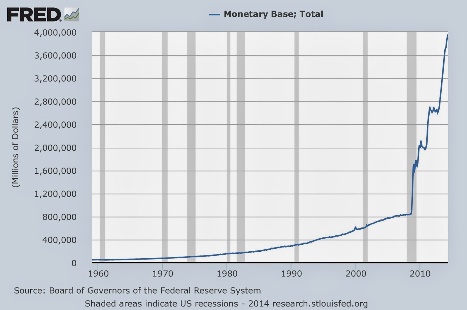
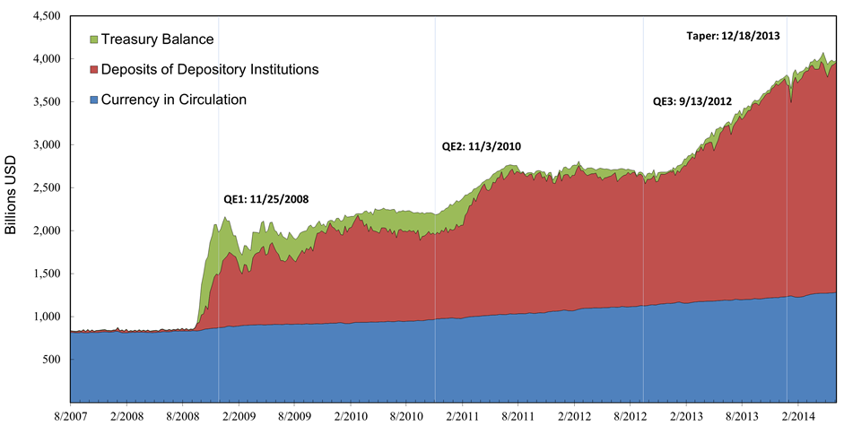
In reality, reversing QE might not be enough. In the model above, I assumed that bonds were of very short duration. In reality, the average duration of the Fed's balance has been extended to about 10 years. What this means is that if interest rates spike up, the Fed is likely to suffer a capital loss on its portfolio. The implication is that it may not have enough assets to buy back all the reserves necessary to keep the price-level in check.
Alternatively, the Fed could increase the interest it pays on reserves. But in this case too, the question is how the interest charges are to be financed? If there is full support from the Treasury, then there is no problem. But if not, then the Fed will (effectively) have to print money (it would book a deferred asset) to finance interest on money. The effect of such a policy would be inflationary.
Finally, how is this related to bank-lending and private money creation? Well, in this model, where banks are assumed to intermediate all assets, broad money is given by M1 = D + P*k. We can eliminate P in this expression by using [16]:
[21] M1 = [ 1 + k/(y-k) ]*D
So when R > 1, reducing z has the effect of increasing capital spending and increasing M1. In the model, young agents want to "borrow" banknotes to finance additional investment spending. But it is not the increase in M1 that causes the price-level to rise. Instead, it is the reduction in the real demand for total government debt that causes the price-level to rise.
Likewise, in the case where R = 1 and then the economy returns to normal, the price-level pressure is coming from the portfolio substitution activity of economic agents: people want to dump their money and bonds in order to finance additional capital spending. The price-level rises as the demand for government securities falls. The fact that M1 is rising is incidental to this process.
